Photonic Quantum Computing

Our natural light source dropping behind the earths curvature in the Baltic sea of chaotic wave functions.
Introduction
To perform a useful calculation with a quantum computer, two problems need to be addressed:
- The Mapping Problem
How to take a task from the real world and formulate it in such a way that it can be solved with a quantum computation.
- The Implementation Problem
How to design, build and configure quantum hardware in such a way that it performs a quantum computation.
The resolution of these problems depends on the task and depends on the hardware, so to retrieve any concrete answers, we need to narrow the scope. In this article we will choose to analyze how to solve a chemistry problem using photonic quantum hardware. Here’s why this is an interesting pair to pick:
Chemistry is a wide field with applications in pharmaceutical development, material design, bat- tery technology, fuel cell research, manufacturing and many other areas. The most efficient way to make discoveries in chemistry, as well as in all of science, is by performing experiments. Run- ning chemistry experiments takes both time and money and the range of possible experiments to run is so vast, that there needs to be a methodology to choose which experiments to perform. This is where computing can help - properties of molecules can be predicted with calculations and the knowledge of those properties enables the chemist to design more informative experiments. However, this almost always comes with a caveat - the more accurate the calculation, the more computational power it demands. If a quantum computer could enable some of those more accurate calculations, then the cost of performing experiments can be reduced and the discovery process can be accelerated. A quantum computer could be the ideal machine for some of these calculations, because all of the processes in chemistry at the atomic level inherently warrant a description based on the laws of quantum mechanics. Such a description is natural to represent on a machine that makes use of those same laws in its principle of operation.
The current notion if quantum computers could be specifically useful and give an advantage over classical computers in a quantum chemistry calculation pipeline is on-going research. [1, 2, 3] Important is to identify exponential scaling behaviour of the computational cost with respect to an increasing molecule size or basis set expansion. Basis sets describe the electronic wave function in form of algebraic equations, e.g. a Gaussian function $$f(x) = a \exp(-\frac{(x-b)^2}{2c^2})$$ . Approximation approaches such as Hartree-Fock (HF) or density functional theory (DFT) make use of such basis sets to turn a partial differential equation (PDE) description of the wave function, the Ψ in the time-independent Schrödinger equation,
$$\frac{-\hbar^2}{2m} \nabla^2\Psi(\vec{r}) + U(\vec{r}) \Psi(\vec{r}) = E \Psi(\vec{r})$$
into algebraic equations.
Therefore these methods are considered as approximations. There exist a whole plethora of such kind of quantum chemistry methods and basis sets to accommodate to the vast space of chemical structures. A lot of experience is needed to choose the right model and suitable basis set for a specific chemical class, or even for a specific chemical structure, followed by a correct analysis of the results. Since larger molecules and more elaborate basis sets will have an effect on the needed computational demand, we speak of this relation as the scaling behaviour. Table 1 shows the scaling behaviour of various classical quantum chemistry models.
Table 1: Various classical approximation methods for quantum chemistry calculations and their scaling behaviour of computational cost with respect to N (size of molecule or expansion of basis set). [2]
| Method | Scaling behaviour |
|---|---|
| DFT | N^3 |
| HF | N^4 |
| MP2 | N^5 |
| MP3, CISD, CCSD | N^6 |
| MP4, CCSD(T) | N^7 |
| MP5,CCSDT | N^8 |
| FCI | 2^N |
The coupled-cluster method with single, double, and perturbative triple excitations, in short CCSD(T), is considered as the “gold standard” of quantum chemical methods to retrieve accurate predictions of practical purposes conforming to experimental measurements of these properties. These kind of coupled cluster (CC) methods converge toward the full configuration interaction (FCI) calculation results being the most demanding to obtain as depicted in Table 1. After this little deep dive into quantum chemistry computations we are going to shift the focus more on photonic hardware aspects and how chemistry related problems can be formulated to be solved with photonic quantum computing algorithms. Photonics (a portmanteau of “photon” and “electronics”) is a hardware platform for processing information with light. If light is prepared in a certain way, as a quantum state, photonics can also be used to process quantum information. There are many reasons to pursue quantum computing on this particular platform. For example, unlike superconducting quantum computers, which are the main focus of companies such as Google and IBM, photonic quantum computers do not require such an immense amount of cooling, currently achievable only with bulky and expensive dilution refrigerators. Also, since light can quickly propagate through free space and optical fibers, photon- ics is the main tool being considered for applications involving quantum communications and the quantum internet. Specifically for photonics, there exist ideas on how to perform distributed and blind quantum computations, which entail a client sending parts of their computation over to a remote quantum server, which performs the calculation for them while being unable to determine what is actually being calculated.
To tackle the mapping and implementation problems, it is first necessary to realize that they are not independent of each other. Figure 1 depicts a schematic relation between these concepts. With conventional computers we have become accustomed to the fact that a software developer does not need to know the inner workings of a computer to create software.

Figure 1: Mapping and implementation relation between chemistry problems and photonic quan- tum computing.
Conversely, the manufacturer of the computer is able to build better components while being confident that the improvements that they make will benefit a wide group of users, regardless of what applications they are building. Quantum computing is currently in a much less mature stage of sophistication, where this is not the case. Both quantum hardware users and providers have to make an effort to communicate their needs and limitations to each other. Ideally, this would be done continuously, such that both the hardware and software are iteratively co-designed to achieve a common goal. At Molecular Quantum Solutions we are working on such kind of a co-design framework together with the Niels Bohr Institute in Copenhagen.
The Mapping Problem
How to take a task from the real world and formulate it in such a way that it can be solved with a quantum computation.
To make the analysis of this problem more manageable, we will further divide it into a sequence of sub-problems:
-
Which real world problem should we pick to solve?
-
Which algorithms could be used to solve this problem?
-
Which parts (if any) of those algorithms could be executed on a quantum computer?
-
What is the procedure for encoding the problem and the algorithm on to quantum hardware?
Problems in Chemistry
In chemistry, there is no shortage of choices. Here is a list of problems in chemistry, for which a quantum computing approach has been proposed or implemented:
- Simulation of electronic structure [4]
- Molecule geometry optimization [5]
- Simulation of vibrational excitations [6]
- Thermodynamic property prediction [7]
- Quantitative structure-activity relations [8]
- Spectroscopic data analysis [9]
- Chemical dynamics [10]
- Reaction mechanism identification [3]
- Drug design [11, 12]
- Catalysis [13]
- Photoemitter design [14]
- Solubility prediction [15]
- Protein folding [16]
- Enzyme design [17, 18]
- Molecular docking [19]
- Conformational search [20]
- Phase diagram generation [21]
- Reaction pathway identification [22]
These problems could be prioritized based on all sorts of metrics, but in the context of picking out one for specifically quantum computation, it makes sense to select the one which would benefit most from a quantum computer. More specifically, it ought to be able to make use of a Noisy Intermediate Scale Quantum (NISQ) computer, which are the devices that we have access to today. Perhaps the most widely studied example is the problem of determining the ground state energy of a molecule, which could be used as a starting point for the simulation of the electronic structure of a molecule. What makes this problem potentially able to benefit from a quantum computer is the fact that it is essentially asking for the solution of the time-independent Schrödinger equation, in the form of a quantum state. Such a problem formulation translates very naturally to a quantum computer, since it is a device specialized in evolving and measuring quantum states. In contrast, representing quantum states on a classical computer demands a lot of resources, because describing a quantum state on a classical machine entails storing it as a vector of complex-valued amplitudes in memory and the dimension of that vector often grows exponentially with the size of the system being studied.
Algorithms and Computational Schemes
After choosing a problem, the second step is to identify an algorithm which would solve that problem. There exists a terminology to classify algorithms based on their relation to quantum computing:
- Classical algorithms
These are designed for and executed on classical computers. Generally, high level program- ming languages are used to describe a step-by-step solution to the problem and compilers are used to translate the higher level code into machine-readable instructions for a classical computer to follow.
- Quantum algorithms
These are designed for quantum computers and most commonly they are formulated as a sequence of instructions that describe how the quantum states (of qubits) should be trans- formed and measured on a quantum computer. Although it is possible to also run classical algorithms on a quantum computer, the term quantum algorithm is usually reserved for those algorithms which specifically make use of the resources that are unique to a quantum computer such as superposition and entanglement.
- Hybrid (quantum-classical) algorithms
hese are algorithms in which parts of the algorithm are classical, whereas other parts are quantum. Running such an algorithm envisions using both a classical and quantum computer, which communicate with each other.
- Quantum inspired algorithms
These are classical algorithms, which have a resemblance to or have been derived from a quantum algorithm. In many cases, these algorithms would likely not have been discovered without the incentive to develop techniques suitable for quantum computing.
Knowing which of these classes a given algorithm belongs to is helpful, because it indicates what kind of hardware is required to perform the calculation. If it is a quantum or hybrid algorithm, then we know that a quantum computer is involved. From the details of the algorithm, it should also be inferred what kind of quantum computer is needed. Mostly, quantum algorithm developers do not describe quantum algorithms in the language of a specific hardware platform, the description is instead given in the context of a computational scheme. To define what that means, we can make the distinction between an algorithm and a computational scheme by examining which question they address:
- Algorithm
If I had a quantum computer, which calculations should I make with it?
- Computation scheme
What actions does my quantum computer need to take to perform a calculation?
The key ingredient here is to ensure compatibility between the two. Each computational step that is required by an algorithm must be translatable into commands that are defined within the computational scheme, otherwise it cannot be executed. In this sense, the computational scheme restricts the set of possible algorithms available to us, but developing algorithms within that restricted set enables us to configure our hardware in an algorithm agnostic way. As long as the computer is able to meet the demands of the computational scheme, any algorithm enabled by that scheme can in principle be executed by the computer. Figure 2 supplements these ideas into the relational scheme constructed in Figure 1.

Figure 2: Relation of quantum algorithms and computational schemes to photonic quantum com- puting
Computational schemes may vary substantially in their degree of abstraction and restrictiveness, so let’s look at some examples.
The Quantum Circuit Model
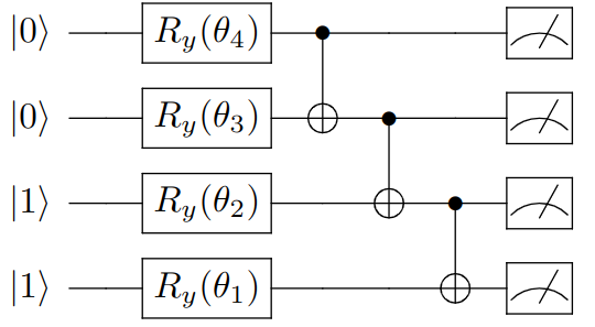
Figure 3: Parameterized quantum circuit with four qubits involving rotation and CNOT gates.
The most popular computational scheme is the quantum circuit model. In the quantum circuit model, the basic building blocks of the quantum computer are assumed to be qubits, and a quan- tum algorithm is executed by applying a sequence of quantum gates to those qubits. Each gate implements a unitary transformation of the quantum state of one or more qubits. The output of the computation is extracted by performing measurements, most often at the very end of the circuit. An example of a quantum circuit is shown in Figure 3. This model is versatile from a hardware perspective, because it does not dictate how exactly the physical implementation of those gates should look like. For example, the unitary transformation needed to implement a two qubit gate on a superconducting quantum computer may involve a sequence of carefully timed microwave pulses, whereas in an optical quantum computer this might be achieved with a static, nonlinear optical element.
Another benefit of the quantum circuit model is that it has been proven to be a universal model of quantum computing. This means that any quantum algorithm which can be conceived of, could in principle be expressed as a quantum circuit. For some quantum algorithms, those circuits may contain quite complicated gates, and it becomes the burden of the hardware developer to provide possibilities to either implement arbitrary quantum gates directly or for a compiler to find a way to approximate them to a satisfactory degree with a combination of simpler ones.
Measurement based Quantum Computing

Figure 4: Measurement based quantum computing model (MBQC). The circles depict qubits and the arrows represent measurements taken in various bases.
Another universal quantum computing scheme is measurement based quantum computing (MBQC), depicted in Figure 4. Unlike the quantum circuit model, there are no quantum gates, only qubits and measurements. It makes use of the fact that measurement changes the state that is being measured, through a process known as wave function collapse. Since the collapse of the wave function is not described by Schrödinger’s equation, it is an irreversible action, which is why some- times MBQC is also called one-way quantum computing. To perform quantum computations with measurements, two main issues need to be addressed:
-
Each measurement collapses superpositions and decreases the degree of entanglement be- tween the qubits. From this perspective, superposition and entanglement can be thought of as resources which are used up during the computation. Measurement based quantum computing requires a highly entangled initial state to begin performing measurements on, since there are no components (e.g. quantum gates) in this model which could generate more of these resources. Such states are called resource states. If the resource state has some par- ticular entanglement structure, it is also sometimes given other names such as cluster state, lattice state, graph state, grid state etc. Some earlier literature uses the terms resource state and cluster state interchangeably. One of the main challenges of MBQC is to engineer the capability to reliably produce these highly entangled resource states.
-
The outcome of every measurement is inherently probabilistic. This means that when de- signing a quantum algorithm for MBQC, the algorithm must either be indifferent to the outcomes or prescribe a method for altering subsequent measurements based on the results of previous ones. The set of instructions that dictate which measurements to perform are sometimes called measurement patterns.
We know that MBQC is universal because various mappings have been found between measurement patterns and quantum circuits. If any quantum circuit can be translated to a measurement pattern, then MBQC must be universal, since the quantum circuit model is universal. Generally, MBQC requires having access to much more qubits and entanglement for the same calculation that a quantum circuit would need, although the overhead is constant.
Ising Machines
Not all computational schemes implement universal quantum computing. One example of a non- universal scheme is the use of an Ising machine. An Ising machine is a machine which can solve only one problem: Given the values of all of the real-valued coefficients hi and Jij , find the configuration s, which minimizes the function
$$E_\text{Ising}(s) &= -\sum h_i s_i - \sum_{ij} J_{ij} s_is_j$$
where each si may take a value of either +1 or −1. Such a machine is not helpful for solving every problem, but it may be very valuable in cases where this specific optimization task is the main computational bottleneck. In this example, the computational scheme is extremely restrictive to the set of quantum algorithms that it is compatible with, and one could even argue that there is not really any room at all for algorithm development on a machine that can perform only one task.
An Ising machine would not even necessarily have to be a quantum device, but there are im- plementations of this in both superconducting and optical devices, which make use of a quantum approach to solve the Ising problem.
Gaussian Boson Sampling
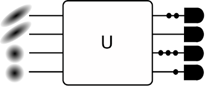
Figure 5: A schematic of a Gaussian boson sampler, where the interferometer is denoted as U . Some inputs are squeezed coherent states (depicted with their elliptical Wigner functions), whereas others are empty (depicted with the circular Wigner function of the vacuum state). The detectors at the output (the popsicles on the far right) count the number of photons (small black circles) arriving from the output.
The final example of a computational scheme that we discuss here is Gaussian Boson Sampling (GBS), shown on 5. GBS is not universal (or at least, no-one has found a way to show that it is) and it is quite restrictive both from the perspective of the problem that it solves and from the hardware that it requires. Instead of qubits, which are discrete, two-level quantum systems, GBS uses Gaussian states of light, which span a continuum of possible quantum states. GBS consists of three main steps:
-
Prepare modes of light in Gaussian states. The definition of a Gaussian state is a state whose Wigner function is described by a Gaussian function.
-
Send these modes through an interferometer.
-
Detect the number of photons at the output of the interferometer.
The task that GBS performs is to measure the distributions of the output for a given interferometer and input of Gaussian modes.
The Implementation Problem
How to design, build and configure quantum hardware in such a way that it performs a quantum computation.
ny quantum system which has at least two quantum states can be used as a qubit, but we have to be careful about which states we choose. There are many different classes of quantum states of light and only some of them are useful for quantum computing purposes, as shown on Figure 6. It is important that we are able to produce and manipulate those states reliably, while avoiding unwanted interactions with other qubits or the environment.

Figure 6: Domains of quantum states of light.
One of the most conceptually simple states to use are single-photon states. One photon can be used to encode a qubit in multiple ways. The main requirement is that the photon can be prepared in two orthogonal quantum states and that we are able to prepare arbitrary superpositions of those two states. Three examples of doing this (also shown in Figure 7) are:
- Time-bin encoding
The arrival time of a photon sent from a source determines which qubit state it represents. Superposition of these states can be generated by sending a photon through a Mach-Zender interferometer.
- Dual-rail encoding
A photon may traverse multiple paths in space and the one that it takes determines the state of the qubit. A superposition of a photon taking two paths can be generated by sending a photon through a beam splitter.
- Polarization encoding
The polarization of a photon determines the state of the qubit. Linear polarizers can be used to generate vertical and horizontal polarization, and a beam splitter can be used to create a superposition of a photon going through either one.

Figure 7: From left to right: time-bin, dual-rail and polarization encoding of qubits with single photons. The black and white variants on each picture represent the two computational basis states of the qubit.
These techniques are not mutually exclusive, so even multiple qubits can be encoded on a single photon. Researchers [23] demonstrated encoding 3 qubits onto a single photon, although in general, the amount of resources required for preparing a multi-qubit photon scales exponentially. If we want to build a scalable quantum computer with single-photons, then all qubits cannot be encoded onto a single photon, which means that we must encode different qubits onto different photons and we need to engineer a way to induce interactions between those photons so that all those qubits can be involved in a single computation. The success of such a computer will then depend on the quality of the single-photon sources which prepare the qubits and the reliability and precision of the interactions.
Single photon sources are devices which are able to emit a single photon on demand, with a known energy, at a specified time and place. The quality of single photon sources are evaluated using the following metrics:
- Efficiency
An ideal photon source would emit a photon every time when requested, but real devices may sometimes fail and not emit any photons. Efficiency characterizes the success rate of the device for emitting photons.
- Purity
An ideal single-photon source would always produce a single-photon state, but real devices may produce slightly different states. For example, upon measurement in the Fock basis, there could be a non-zero probability for the state to collapse to a two photon state. The purity of a photon source characterizes how close the produced state is to a single-photon state.
- Indistinguishability
An ideal photon source would emit indistinguisbale photons, which means that all the photons it emits need to be identical in every respect. This includes attributes such as frequency and the relative time and place where the photon is emitted from when the source is used. Indistinguishability is not only important for consistency of results, it plays a fundamental role in many quantum-mechanical interactions, which are required in quantum computing protocols. Photon indistinguishability can be evaluated by observing the Hong-Ou-Mandel effect.
High quality single-photon sources are difficult to build. This partially motivates research into other quantum states of light which may be easier to generate. An important class of examples are Gaussian states of light, in particular squeezed states [24]. These can be more reliably generated, but they cannot be regarded as two-level systems, which means that there is no straightforward way to use these as qubits. Nonetheless, quantum computing applications can be developed specif- ically for these states, with Gaussian boson sampling being the prime example.
Interestingly, the Gaussian boson sampling setup can be used with minimal modifications to create GKP qubits, which are qubits that are based on GKP states of light [25]. Although the mech- anism for this is inherently probabilistic, generation of GKP qubits may be worthwhile, because they offer a method for error mitigation [26], in a way which is inaccessible for qubits based on photon number states.
In summary, there are many possible quantum states of light which can be used to implement quantum computations and even within a single choice of state, there are various ways in which they can be employed to construct useful quantum computing capabilities. It is an active area of research to identify new ways to process quantum information with light and to improve the performance of existing methods.
So Long, and Thanks for All the Photons
This blog article was an attempt by us at Molecular Quantum Solutions to give an introduction to photonic quantum computing. Together with our partners in the PhotoQ Grand Solutions project funded by the Innovation Fund Denmark we are working on a full stack photonic quantum computer implementation.

Figure 8: The PhotoQ logo for the Grand Solutions project funded by the Innovation Fund Denmark.
We aim to describe the detailed work performed within the PhotoQ project in more detail with a follow up publication in form of another blog article and/or research publication.
References
[1] Seunghoon Lee, et al., “Is there evidence for exponential quantum advantage in quantum chemistry?” 2022. https://arxiv.org/abs/2208.02199
[2] Michael Kühn, Sebastian Zanker, Peter Deglmann, Michael Marthaler, and Horst Weiß, “Accuracy and resource estimations for quantum chemistry on a near-term quantum computer” Journal of Chemical Theory and Computation, vol. 15, no. 9, pp. 4764–4780, 2019. https://doi.org/10.1021/acs.jctc.9b00236
[3] Markus Reiher, Nathan Wiebe, Krysta M Svore, Dave Wecker, and Matthias Troyer, “Elucidating reaction mechanisms on quantum computers” Proceedings of the national academy of sciences, vol. 114, no. 29, pp. 7555–7560, 2017. https://doi.org/10.1073/pnas.161915211
[4] Rongxin Xia, Quantum Computation For Electronic Structure Calculations. PhD thesis, Pur- due University Graduate School, 2020. https://doi.org/10.25394/PGS.13302965.v1
[5] Alain Delgado, et al., “Variational quantum algorithm for molecular geometry optimization” Physical Review A, vol. 104, no. 5, p. 052402, 2021. https://doi.org/10.1103/PhysRevA.104.052402
[6] Soran Jahangiri, Juan Miguel Arrazola, Nicolás Quesada, and Alain Delgado, “Quantum algorithm for simulating molecular vibrational excitations” Physical Chemistry Chemical Physics, vol. 22, no. 44, pp. 25528–25537, 2020. https://doi.org/10.1039/D0CP03593A
[7] Spencer T Stober, et al., “Considerations for evaluating thermodynamic properties with hybrid quantum-classical computing work flows” Physical Review A, vol. 105, no. 1, p. 012425, 2022. https://doi.org/10.1103/PhysRevA.105.012425
[8] Teppei Suzuki and Michio Katouda, “Predicting toxicity by quantum machine learning” Jour- nal of Physics Communications, vol. 4, no. 12, p. 125012, 2020. https://doi.org/10.1088/2399-6528/abd3d8
[9] Chee-Kong Lee, Chang-Yu Hsieh, Shengyu Zhang, and Liang Shi, “Simulation of condensed- phase spectroscopy with near-term digital quantum computers” Journal of Chemical Theory and Computation, vol. 17, no. 11, pp. 7178–7186, 2021. https://doi.org/10.1021/acs.jctc.1c00849
[10] Chee-Kong Lee, Chang-Yu Hsieh, Shengyu Zhang, and Liang Shi, “Variational quantum sim- ulation of chemical dynamics with quantum computers” Journal of Chemical Theory and Computation, vol. 18, no. 4, pp. 2105–2113, 2022. https://doi.org/10.1021/acs.jctc.1c01176
[11] Kushal Batra, et al., “Quantum machine learning algorithms for drug discovery applications” Journal of chemical information and modeling, vol. 61, no. 6, pp. 2641–2647, 2021. https://doi.org/10.1021/acs.jcim.1c00166
[12] Maximillian Zinner, et al., “Quantum computing’s potential for drug discovery: Early stage industry dynamics” Drug Discovery Today, vol. 26, no. 7, pp. 1680–1688, 2021. https://doi.org/10.1016/j.drudis.2021.06.003
[13] Vera von Burg, et al., “Quantum computing enhanced computational catalysis,” Physical Review Research, vol. 3, no. 3, p. 033055, 2021.
[14] Qi Gao, et al., “Applications of quantum computing for investigations of electronic transitions in phenylsulfonyl-carbazole tadf emitters,” npj Computational Materials, vol. 7, no. 1, pp. 1–9, 2021. https://doi.org/10.1038/s41524-021-00540-6
[15] Davide Castaldo, Soran Jahangiri, Alain Delgado, and Stefano Corni, “Quantum simulation of molecules in solution” arXiv preprint arXiv:2111.13458, 2021. https://doi.org/10.48550/arXiv.2111.13458
[16] Anton Robert, Panagiotis Kl Barkoutsos, Stefan Woerner, and Ivano Tavernelli, “Resource- efficient quantum algorithm for protein folding” npj Quantum Information, vol. 7, no. 1, pp. 1–5, 2021. https://doi.org/10.1038/s41534-021-00368-4
[17] Hai-Ping Cheng, Erik Deumens, James K Freericks, Chenglong Li, and Beverly A Sanders, “Application of quantum computing to biochemical systems: A look to the future” Frontiers in Chemistry, vol. 8, p. 587143, 2020. https://doi.org/10.3389/fchem.2020.587143
[18] Vikram Khipple Mulligan, et al., “Designing peptides on a quantum computer” BioRxiv, p. 752485, 2020. https://doi.org/10.1101/752485
[19] Leonardo Banchi, Mark Fingerhuth, Tomas Babej, Christopher Ing, and Juan Miguel Arra- zola, “Molecular docking with gaussian boson sampling” Science advances, vol. 6, no. 23, p. eaax1950, 2020. https://doi.org/10.1126/sciadv.aax1950
[20] DJJ Marchand, et al., “A variable neighbourhood descent heuristic for conformational search using a quantum annealer” Scientific reports, vol. 9, no. 1, pp. 1–13, 2019. https://doi.org/10.1038/s41598-019-47298-y
[21] Akhil Francis, Ephrata Zelleke, Ziyue Zhang, Alexander F Kemper, and James K Freericks, “Determining ground-state phase diagrams on quantum computers via a generalized applica- tion of adiabatic state preparation” Symmetry, vol. 14, no. 4, p. 809, 2022. https://doi.org/10.3390/sym14040809
[22] Philipp Hauke, Giovanni Mattiotti, and Pietro Faccioli, “Dominant reaction pathways by quantum computing” Physical Review Letters, vol. 126, no. 2, p. 028104, 2021. https://doi.org/10.1103/PhysRevLett.126.028104
[23] Kumel H Kagalwala, Giovanni Di Giuseppe, Ayman F Abouraddy, and Bahaa EA Saleh, “Single-photon three-qubit quantum logic using spatial light modulators” Nature communications, vol. 8, no. 1, pp. 1-11, 2017. https://doi.org/10.1038/s41467-017-00580-x
[24] Alexander I Lvovsky, “Squeezed light” Photonics: Scientific Foundations, Technology and Applications, vol. 1, pp. 121-163, 2015. https://doi.org/10.1007/978-3-319-19273-4_8
[25] J Eli Bourassa, et al., “Blueprint for a scalable photonic fault-tolerant quantum computer” Quantum, vol. 5, p. 392, 2021. https://doi.org/10.22331/q-2021-02-04-392
[26] Kosuke Fukui, Akihisa Tomita, Atsushi Okamoto, and Keisuke Fujii, “High-threshold fault-tolerant quantum computation with analog quantum error correction” Physical review X, vol. 8, no. 2, p. 021054, 2018. https://doi.org/10.1103/PhysRevX.8.021054