Run a Graph Neural Network via Cebule or Kubeflow
MQS Documentation
This blog is now defunct. Head over to https://docs.mqs.dk
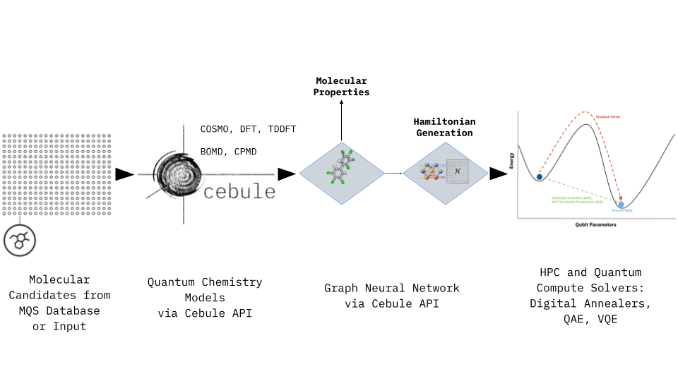
Accessing the MQS Graph Neural Network (GNN) Model through the Cebule API
We have now added an updated and further developed Graph Neural Network (GNN) model to the Cebule Application Programming Interface (API) where several endpoints allow to create/extend/delete a data set, train a GNN model and use the trained model as a prediction model. The endpoints of the API can be accessed via the Python SDK (https://gitlab.com/mqsdk/python-sdk) with the task types:
- GNN_DATASET_CREATE
- GNN_DATASET_DELETE
- GNN_DATASET_EXTEND
- GNN_TRAIN
- GNN_PREDICT
Here is an example to create a dataset for a training task:
|
|
The following code snippet shows how to extend this dataset with some data once the previous task has completed:
|
|
You can repeatedly call the above task to construct your dataset in chunks.
To view chunks of your created dataset (from a start index to an end):
|
|
The above task will return the last two molecules out of the 3 which were added to “dataset_a”.
Deleting a dataset again is also possible:
|
|
After the dataset create/extend tasks have been completed you can start training the GNN model:
|
|
And when the training task has been completed, you will be able to apply the GNN model for predicting the target property for a dataset with new molecular structures:
|
|
We have already utilized the MQS GNN as a toxicity classifier, or as a Hamiltonian generator. The Hamiltonian generator allows to retrieve the needed problem description of large molecules (approx. 500 g/mol) to be solved by digital annealers, quantum annealers or variational quantum eigensolver (VQE) methods. A complete Jupyter notebook with all the TaskType examples above can be found under the following link: https://gitlab.com/mqsdk/python-sdk/-/blob/main/notebooks/8_GNN.ipynb
Please contact us via contact (at) mqs (dot) dk, if you would like to have an onboarding session how the combination of our quantum chemistry models and the GNN model can be utilized for your use-case application.
The visualisation at at the top of this blog article shows the individual steps of this holistic pipeline and the framework allows to tackle many different pharma, biopharma, chemical and materials applications. The following table gives an overview of the domain specific use-cases:
| Use-case Domain → | Formulation Development & Product Design | Upscaling & Process Simulations | Materials Design |
|---|---|---|---|
| Properties → | Solubility, Stability, Toxicity, Viscosity | Vapour-Liquid Equilibrium (VLE) | HOMO-LUMO Gap, Ground & Excited States |
| Binding Analysis | Liquid-Liquid Equilibrium (LLE) | Seebeck Coefficient | |
| Solid-Liquid Equilibrium (SLE) | Solubility, Phase Stability | ||
| Use-case Examples → | (Bio)Pharma Solubility in Multi-compound Mixtures | Crystallizer Design for Purification Processes | OLED Materials |
| Toxicity Checks in Pharma & Chemical Product Development | Solvents Analysis for CO2 Capture & CO2 Utilization Processes | Energy Storage Materials | |
| Human, Animal and Environmental Safety | Liquid-Liquid Chromatographic Separation | High-Entropy Alloys | |
| Beauty Care Product Design | Property data for Computational Fluid Dynamics (CFD) | Catalyst Design | |
| Integrated Drug Discovery & Formulation Analysis | Anti-corrosion and Functional Coatings |
In the next section we present an example how to predict the HOMO-LUMO gap with the GNN model via Kubeflow (https://dashboard.mqs.dk/subscriptions). Kubeflow is the second option apart from the MQS Python SDK how to utilize the MQS model library.
Introduction
In the previous tutorial, we saw how a fine-tuned DelFTa EGNN model [1] on PCB data from the PubChemQC PM6 quantum chemistry dataset [2] can result in more accurate HOMO-LUMO gap (toxicity indicator) prediction of PCB molecules. This also eliminated outlier predictions that were previously present with a pre-trained DelFTa model on the QMugs dataset [3].
In this tutorial, we first present a novel graph neural network: a Matrix-completed Graph Neural Network (MCGNN); and compare its PCB HOMO-LUMO gap prediction to the DelFTa model by first training it on the ~2 million molecules in QMugs, and then fine-tuning it with PCB data from PubChemQC PM6. This MCGNN slightly outperforms DelFTa on the PCB dataset after fine-tuning.
Furthermore, we then demonstrate how to fine-tune your own MCGNN and DelFTa models on Kubeflow, which is incorporated in the MQS Dashboard Machine Learning tier. One can then run predictions with the fine-tuned model on arbitrary molecules. All parts of the ML pipeline have been modularized to allow the user to tailor the models based on their use-case and dataset choice.
The following molecular properties/information can be predicted with our models:
- HOMO-LUMO gaps - available via MCGNN and DelFTa with MQS Dashboard ML subscription
- Hamiltonians (total energy functions)
- Activity coefficients
- Critical physical properties (critical temperature, critical pressure, acentric factor)
- Solubilities
- Phase equilibria (VLE, SLE, LLE)
Contact us for more information with respect to these properties. Currently only the HOMO-LUMO gap model is provided in the ML tier of the MQS Dashboard.
Currently the following data sets can be accessed via the MQS Dashboard:
- PubchemQC PM6
- QMugs
MCGNN model overview
Graph Neural Networks (GNNs) are neural networks specifically designed to operate on graph-structured data. A molecule can for example be mapped to a GNN where a message-passing layer facilitates information exchange and aggregation between connected nodes (atoms), enabling nodes to update their representations based on messages received from neighboring nodes (bonded atoms). This enables effective modelling of relational structures and improves the network’s ability to learn from graph-structured data.
Our Matrix-completed GNN (MCGNN) combines (with modifications) two techniques: a Directed Message Passing Neural Network (D-MPNN) [4] and a Matrix Completion Method (MCM) [5].
A D-MPNN involves constraining the message-passing layer of a GNN to prevent messages being passed back and forth between the same nodes in the graph; this problem creates noise in normal message-passing layers. The D-MPNN has directed edges betweens nodes to achieve this, and passes messages along these directed edges. Our D-MPNN is the first step of the MCGNN, taking in molecular properties such as atom type, atom 3D coordinates, and bond information similar to DelFTa’s input data, and outputting overall graph features for a molecule as a vector.
Our model also uses a MCM method originally designed for activity coefficient prediction of solutes in ionic liquids that we have modified to fit with our D-MPNN output. The MCM takes in the molecule graph feature vector outputted from the D-MPNN. It uses multiple neural network layers, in a multi-layer perceptron (MLP), to ultimately predict a molecular property like the HOMO-LUMO gap value.
In summary, for each datapoint, the MCGNN acts in the following way:
- 3D molecular structures are the input to the model
- D-MPNN outputs aggregated graph features for the molecular structures
- MCM outputs a specific molecular property for the graph features
The MCGNN training and test pipeline can be summarized with the following steps:
- Collect 3D molecular structures and other relevant training data as features for training
- Train MCGNN (D-MPNN and MCM) to predict a molecular property based on the training data, validating its progress with a validation dataset after every epoch
- Test MCGNN with test data set
MCGNN performance compared to DelFTa
We evaluate the performance of both a MCGNN trained on HOMO-LUMO Gap data from the QMugs dataset and a fine-tuned MCGNN on the PubchemQC PM6 data for the 194 PCBs analyzed in the previous blog article.
The PCB prediction performance of the fine-tuned and pre-trained DelFTa models from the previous blog article is in Figure 1 and Figure 2 below.
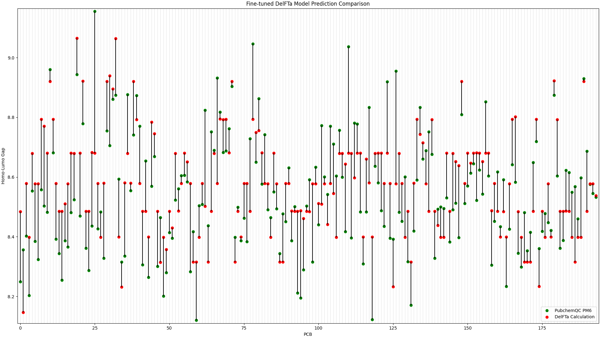 Figure 1: Fine-tuned DelFTa Model Prediction Comparison
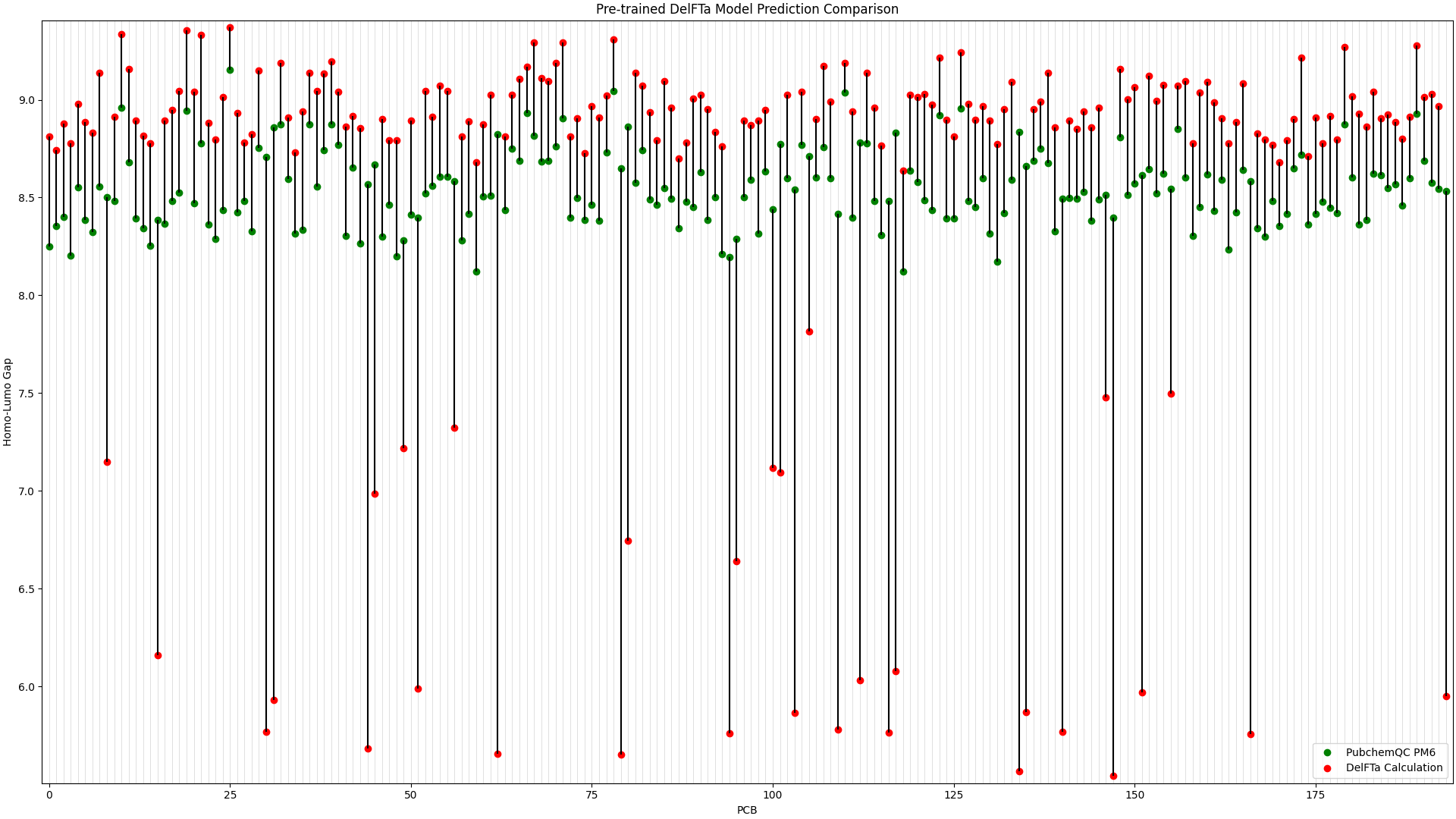 Figure 2: Pre-trained DelFTa Model Prediction Comparison
Recall that the test data of 39 molecules (none of which were outlier predictions) does not hold any training data points from the fine-tuning step. The pre-trained DelFTa model had a mean absolute error for the test data of 0.41 eV, while the fine-tuned DelFTa model had a mean absolute error of 0.11 eV.
We evaluate the MCGNN fine-tuned and pre-trained (trained only on QMugs) models in the same way in Figure 3 and Figure 4 below.
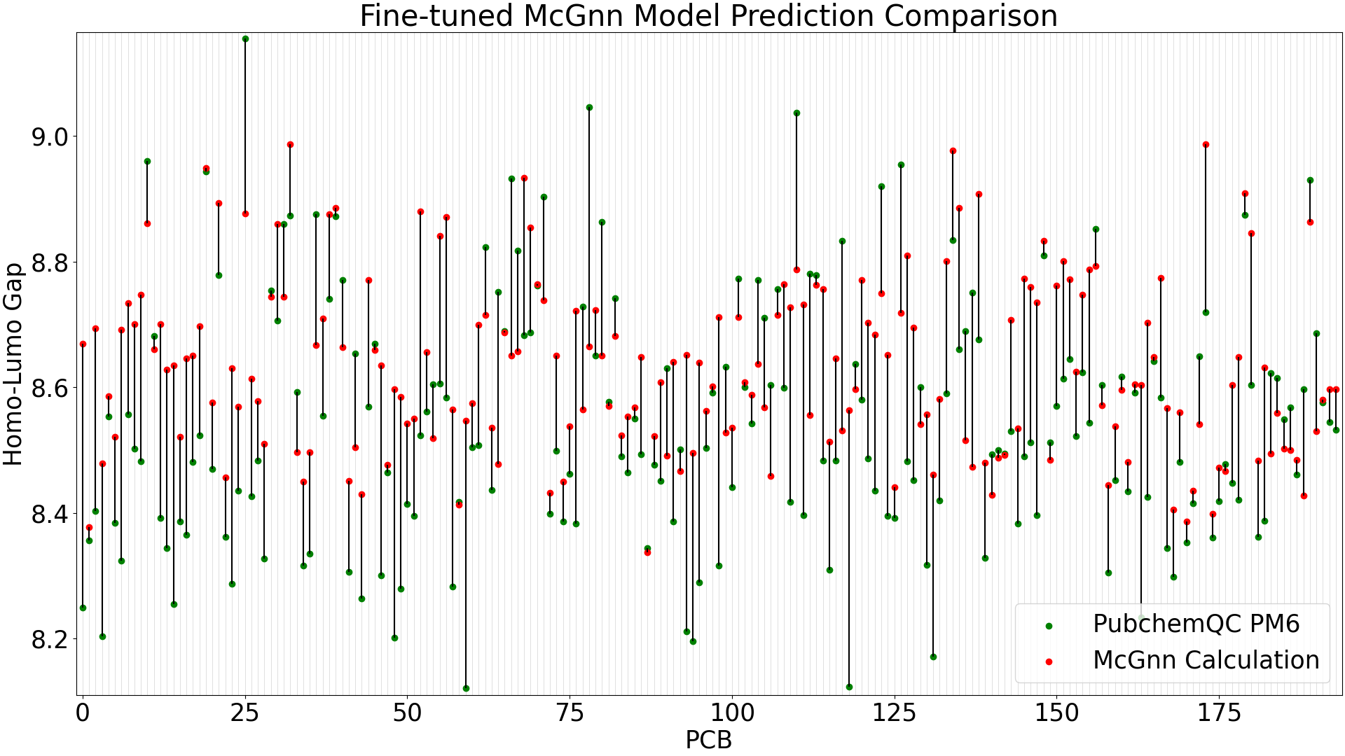 Figure 3: Fine-tuned MCGNN Model Prediction Comparison
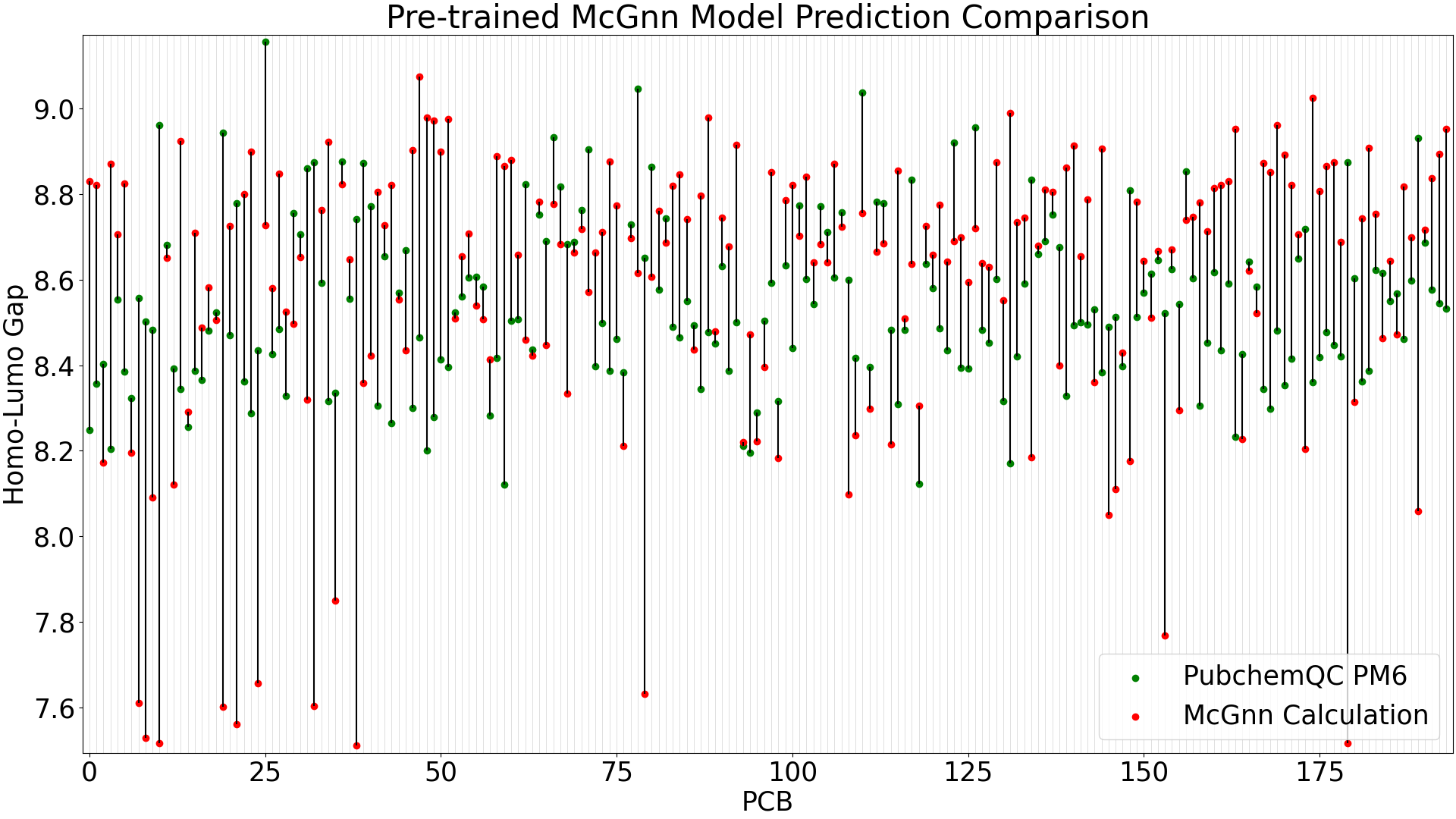 Figure 4: Pre-trained MCGNN Model Prediction Comparison
When running predictions with the test data (39 molecules), the pre-trained MCGNN model shows a mean absolute error of 0.35 eV, while the fine-tuned MCGNN has significant improvement with a mean absolute error of 0.10 eV.
The larger-error predictions in the pre-trained MCGNN plot (Figure 4) are still less than DelFTa’s pre-trained model predictions (Figure 2), and we can see that the accuracy of both the pre-trained and fine-tuned MCGNN models outperform (pre-tained) and slightly outperform (fine-tuned) the DelFTa model counterparts.
Fine-tuning a model via Kubeflow
Anyone with the Machine Learning tier MQS subscription can fine-tune a MCGNN or DelFTa model in Kubeflow via the MQS Dashboard and choose a query to select molecules to train on. Here, we will use the following query to grab 194 PCBs from the PubchemQC PM6 and QMugs data sets (although the data for fine-tuning will be solely taken from the PubchemQC PM6 data set):
|
|
Using this query, we will fine-tune a MCGNN model to predict the HOMO-LUMO gap based on the PCBs’ 3D molecular structures. The Kubeflow training pipeline will fetch the PCB data using the MQS API and then train the model with it.
To run the Kubeflow training pipeline, follow these steps from the MQS Kubeflow Dashboard:
-
Create an experiment in
Experiments (KFP) -> Create experiment, entering a name and then hittingNext: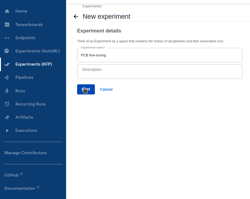
-
Run the training pipeline
2.1. Go to
Runs -> Create run2.2. For
Pipeline, select themodel_trainingpipeline underSharedpipelines2.3. For
Experiment, select the experiment you just created2.4. Give your model an ID in
model_idso you can reference it after training. The ID cannot bedelftaormcgnn(model_nameoptions). We do not support overwriting existing model IDs with new trained models2.5. Choose between
mcgnnordelftaformodel_name. We will demonstrate training a MCGNN model2.6. Enter the PCB query above for
query. Note that datasets for fine-tuning are limited to 1000 or less molecules2.7. Enter
homo_lumo_gapfortarget_property. More properties will be supported soon.2.8. Finally, hit
Startto start the training procedure.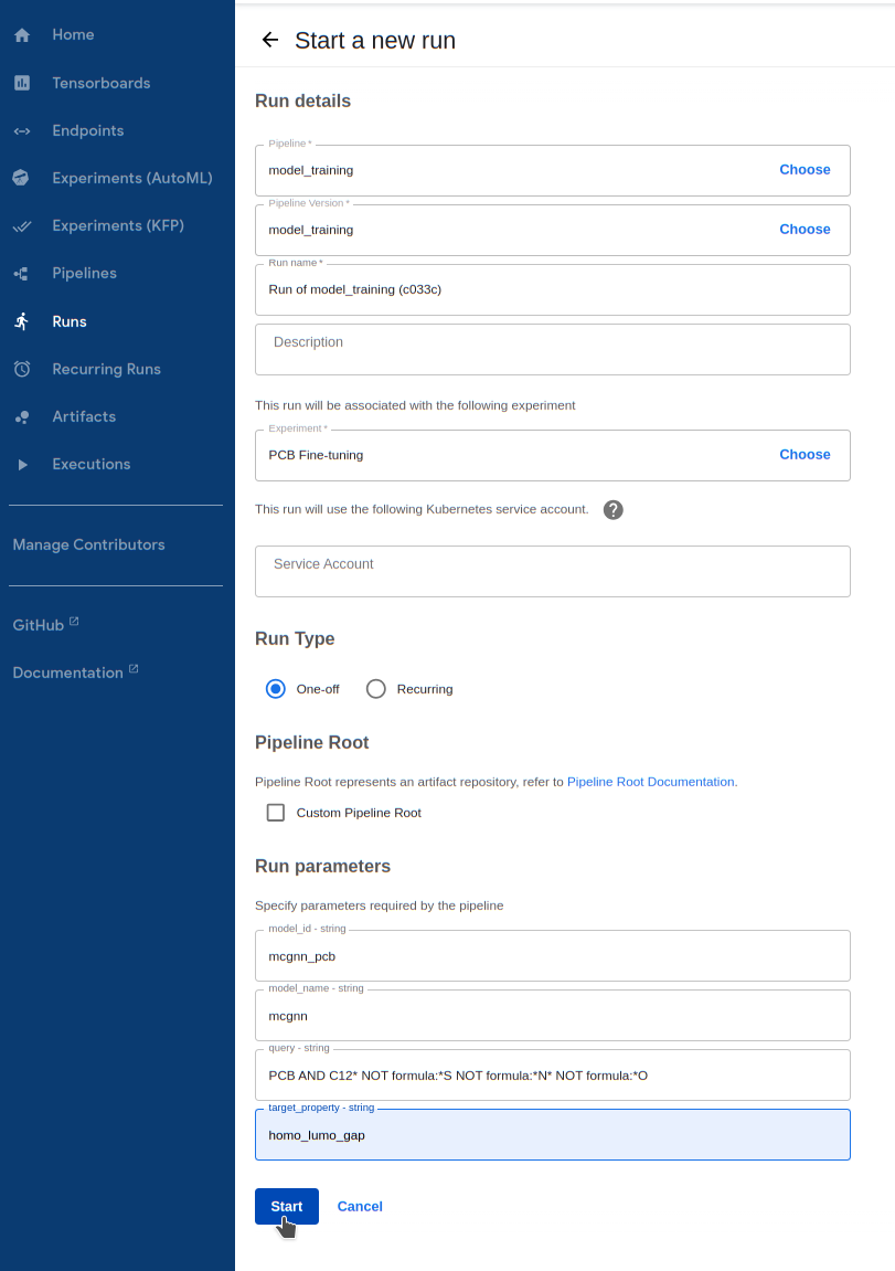
-
Wait for the training procedure to complete and display green marks on the following components. If the pipeline fails (likely due to invalid input), click on the failed component and view its
Logsto see the error message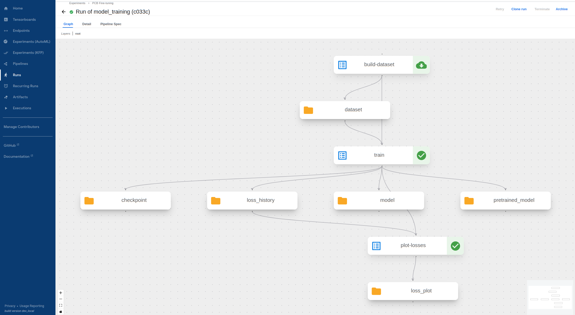
-
Visualize outputs! The successful training step creates a dataset text file, model files, as well as a loss history file and plot. Let’s take a look at the loss history plot by going to
Artifactsand clicking on theURIforloss_plot: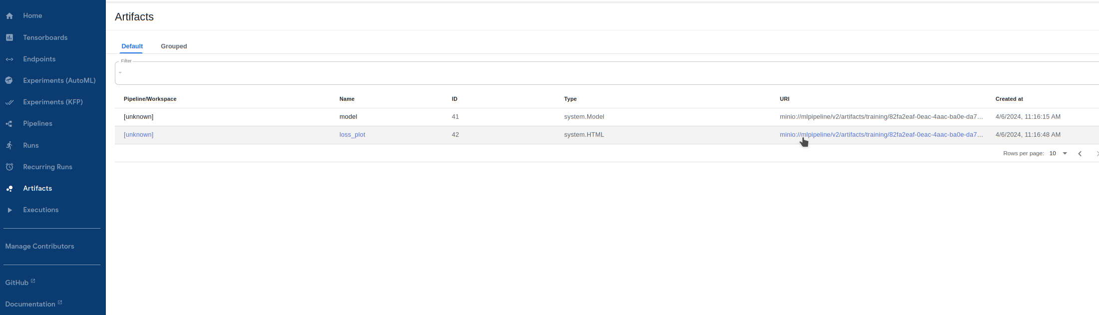
-
This will open up HTML file source code which we can save locally with
ctrl-S. A current limitation with Kubeflow is that all output files are saved as.txtfiles, so when saving this file, please change the extension of theloss_plotfile from.txtto.html. Then, view this file in browser withctrl-Oand then selecting the downloaded file. This displays a plot of training/validation mean squared error (MSE) loss versus number of training epochs: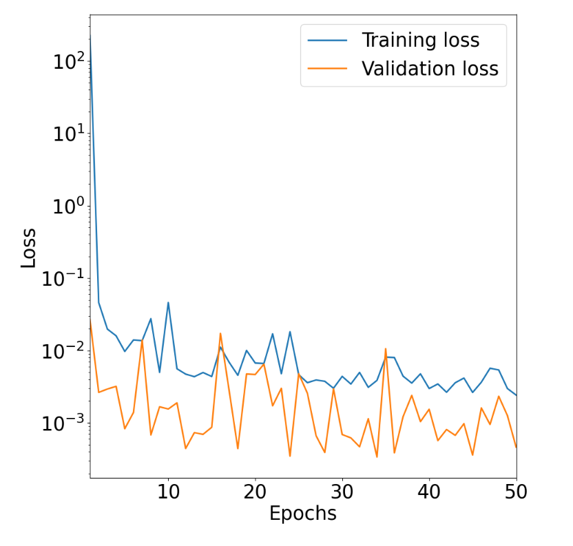
-
Similarly, you can view the
loss_historytext file by downloading it from theArtifactspage (no need to convert it to.html). Note that visualization for text and HTML files should be supported from the Kubeflow UI in the future so downloading will not be required.
Prediction with trained model via Kubeflow
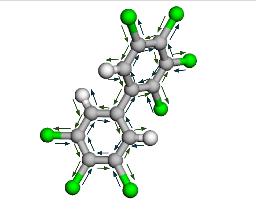
Once the model has been trained we can run a prediction with arbitrary molecules, although one has to evaluate carefully how well the model covers the prediction of molecules that are not very similar to the training data, for example molecules not being part of the same molecule class which the model has been trainined on. Figure 5 and Figure 6 show the two PCBs 2,3,3’,4,4’,5,5’-Heptachlorobiphenyl and 3,3’,4,5-Tetrachlorobiphenyl, which we will run prediction on with the MCGNN we just fine-tuned.
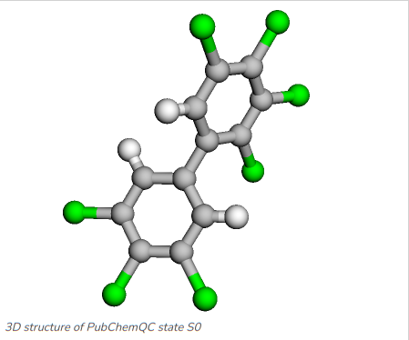
Figure 5: 2,3,3’,4,4’,5,5’-Heptachlorobiphenyl: C1=C(C=C(C(=C1Cl)Cl)Cl)C2=CC(=C(C(=C2Cl)Cl)Cl)Cl
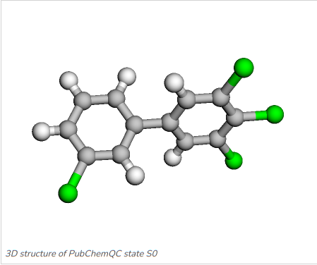
Figure 6: 3,3’,4,5-Tetrachlorobiphenyl: C1=CC(=CC(=C1)Cl)C2=CC(=C(C(=C2)Cl)Cl)Cl
To select these molecules for prediction, the following comma-separated list of the PCBs’ SMILES definition is applied:
|
|
The prediction pipeline will read in and geometry-optimize these molecule SMILES before predicting the HOMO-LUMO gap, which allows us to run predictions on molecules that are not in the database as well.
-
Run the prediction pipeline
1.1. Go to
Runs -> Create run1.2. For
Pipeline, select themodel_predictionpipeline underSharedpipelines1.3. For
Experiment, select the experiment you created earlier1.4. Enter your model’s ID in
model_id. If you wanted to run prediction on a pre-trained model without fine-tuning, you can choose fromdelftaandmcgnnfor this field1.5. Choose the
model_nameyou fine-tuned earlier, betweenmcgnnordelfta. We trained a MCGNN model in this tutorial1.6. Enter the PCB SMILES list above for
smiles_csv1.7. Finally, hit
Startto kick it off!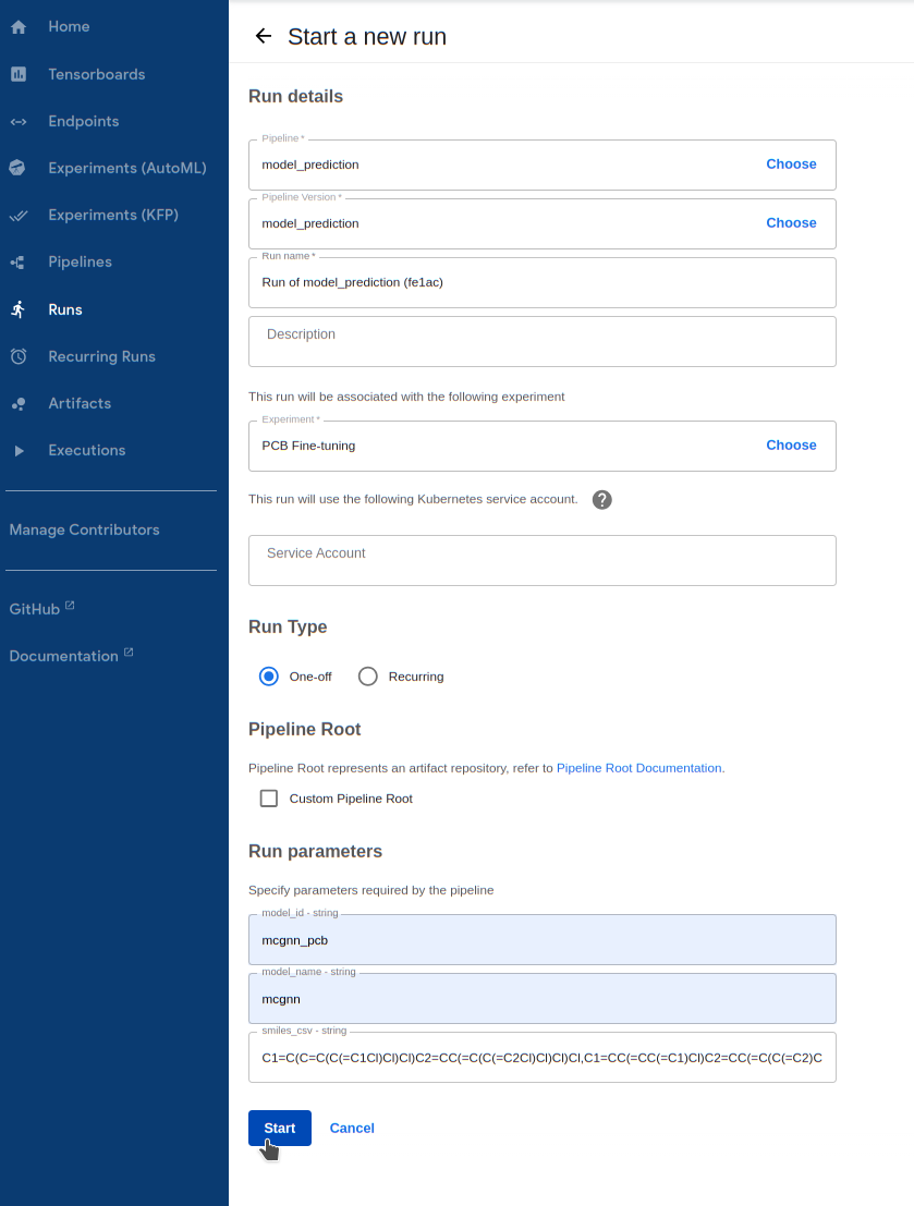
-
Wait for the prediction procedure to complete and display a green mark on the following component. If the pipeline fails (likely due to invalid input), click on the failed component and view its
Logsto see the error message. Note that amodeloutput shows up here, but this is just because the model data is downloaded onto the Kubeflow worker for prediction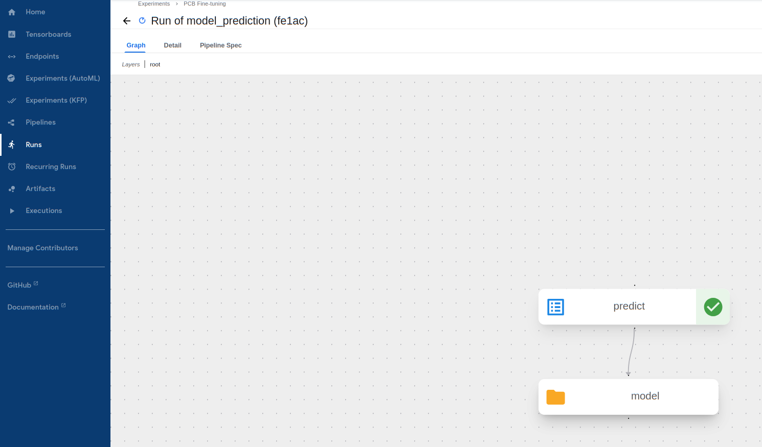
-
See the predicted HOMO-LUMO Gap for each molecule! We can see this by clicking on the
predictcomponent and looking at theOutput: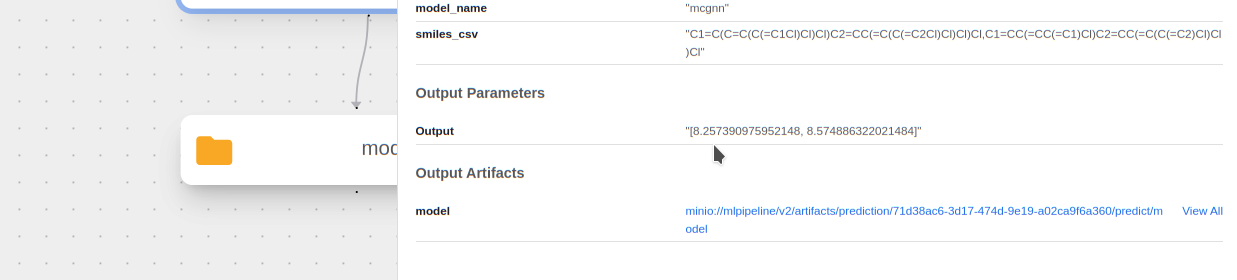
-
The actual HL gap values for these PCBs are 8.23 eV and 8.57 eV respectively. It makes sense that the model predicted extremely well with these as they are in the training data.
We hope we showed you that our custom MCGNN model, as well as our procedure for fine-tuning models with Kubeflow Pipelines, can be of value for interesting machine learning studies with molecular quantum information.
You are always welcome to reach out if you have any feedback, questions, ideas or even collaboration projects to push this kind of work and research further (contact (at) mqs [dot] dk).
References
[1] K. Atz, C. Isert, M. N. A. Böcker, J. Jiménez-Luna & G. Schneider; Δ-Quantum machine learning for medicinal chemistry; ChemRxiv (2021); http://doi.org/10.26434/chemrxiv-2021-fz6v7-v2
[2] M. Nakata, T. Shimazaki, M. Hashimoto, and T. Maeda; PubChemQC PM6: Data Sets of 221 Million Molecules with Optimized Molecular Geometries and Electronic Properties; J. Chem. Inf. Model. (2020), 60, 12, 5891–5899; https://doi.org/10.1021/acs.jcim.0c00740
[3] C. Isert, K. Atz, J. Jiménez-Luna & G. Schneider; QMugs, quantum mechanical properties of drug-like molecules; Sci Data 9, 273 (2022); https://doi.org/10.1038/s41597-022-01390-7
[4] K. Yang, K. Swanson, W. Jin, C. Coley, P. Eiden, H. Gao, A. Guzman-Perez, T. Hopper, B. Kelley, M. Mathea, A. Palmer, V. Settels, T. Jaakkola, K. Jensen & R. Barzilay; Analyzing Learned Molecular Representations for Property Prediction; Journal of chemical information and modeling 59.8 (2019): 3370-3388; https://arxiv.org/pdf/1904.01561v2.pdf
[5] J. G. Rittig, K. B. Hicham, A. M. Schweidtmann, M. Dahmen, A. Mitsos; Graph Neural Networks for Temperature-Dependent Activity Coefficient Prediction of Solutes in Ionic Liquids; Computers & Chemical Engineering 171, 108153 (2023); https://arxiv.org/pdf/2206.11776.pdf