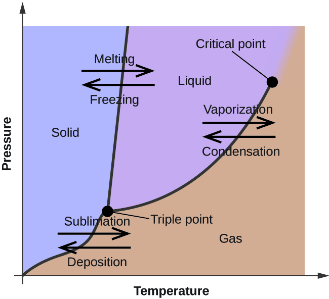
Figure 1: Temperature-Pressure phase diagram [1]

Introduction to thermodynamics

The chemical potential is an important theoretical quantity in the field of thermodynamics and describes the change in energy of a chemical system of multiple components where the composition of a system is under change.

The composition of atoms or molecules in the system can change due to a reaction or due to a flux between the system/phase boundaries. Common examples of such chemical phenomena can be observed in our environment or in industrial processes (Figure 1).

The chemical potential can be related to thermodynamic state functions, namely internal energy \(U(S,V)\), enthalpy \(H(S,p)\), Helmholtz energy \(F(T,V)\), Gibbs enery \(G(T,p)\):

$$dU = TdS − pdV + \sum_i \mu_i dni$$

$$dH = TdS − VdT + \sum_i \mu_i dni$$

$$dF = -pdV - TdS + \sum_i \mu_i dn_i$$

$$dG = Vdp - SdT + \sum_i \mu_i dn_i$$

and one can derive that:

$$\mu_i = (\frac{\delta G}{\delta n_i})_{p,T,n_j}$$

Phase equilibria calculations such as vapour liquid equilibria (VLE), liquid liquid equilibria (LLE), solid liquid equilibria (SLE) are states where the chemical potentials of all the phases are equal: $$\mu_i^j = \mu_i^l$$

With this quick recap of some basic thermodynamic equations we will move on to discuss the theory of implicit solvation models and circle back to the connection between solvation models and thermodynamic properties in the end of the solvation models section.

Solvation models

When considering the environment of an atom or molecule in solution, then the electronic effect of the atoms/molecules surrounding an atom/molecule of interest needs to be taken into account.

Implicit solvation models describe this interaction between a solute and a solvent with considering a polarizable continuum (also called dielectric medium). This electronic spatial profile of molecules allows to map a profile of positive and negative charge distributions on a specific surface around the solute molecule. This profile is called the apparent surface charge (ASC) density \(\sigma(\vec{s})\) and defines a border between the solute and the continuum of the solvent. The polarity of the solvent will have an influence on the ASC density and the polarity is defined with the dielectric constant \(\epsilon(\vec{r})\).

The electrostatic solvation energy of a molecule in solutions is defined as:

$$G^{el}_{solvation} = \frac{1}{2} \int_s \sigma(\vec{r}) \phi(\vec{r})$$

and is the change in energy when transferring the molecule under consideration from the gas phase into the solution/solvent(s) phase. The integration is performed over the solute surface points \(s\).

To retrieve the before mentioned apparent surface charge (ASC) density \(\sigma(\vec{r})\) of the solute molecule, the Poisson equation has to be solved [2]:

$$ \nabla [\epsilon(\vec{r}) \nabla \phi(\vec{r})] = - 4 \pi \rho(\vec{r})$$

Where the equation simplifies with \(\epsilon(r) = 1\) within the solute molecule cavity to:

$$ \nabla^2 \phi(\vec{r}) = - 4 \pi \rho(\vec{r})$$

and with \(\epsilon(r) = \epsilon\) (set to a constant value, e.g. to 80 for water) outside of the solute cavity to:

$$ \epsilon \nabla^2 \phi(\vec{r}) = 0 $$

There exist different ways how the Poisson equation can be solved where the electrostatic surface around the molecule is dissected into smaller pieces (tesserae). The Poisson equation is then being solved in combination with a tesserae dissection routine.

In this article we present the DPCM, CPCM/COSMO and IPCM/IEFPCM models which differ based on the implemented boundary conditions. Important to highlight is that the DPCM model relies on the net electric field, \(E_n\), and the COSMO and IEFPCM models depend only on the net potential (\(\phi(s)\)) at the cavity surface of a given solute molecule [3]. IEFPCM reduces to the COSMO model when \(\epsilon\) approaches infinity [4].

To solve the Poisson equation numerically and to provide a general mathematical formulation, one can recast the equation in matrix form:

$$\vec{q} = \mathbf{K} \vec{f} $$

with \(\vec{q}\) storing the unknown cavity surface charges, \(\mathbf{K}\) (the solvent response matrix) being a square matrix storing the information about the geometry (tesserae location, area) and dielectric information of the medium.

\(\mathbf{K}\) is defined by the matrices/operators \(\mathbf{A}\), \(\mathbf{D}\) and \(\mathbf{S}\) presented later. \(\vec{f}\) holds the normal component of the electrostatic quantity at the tesserae. Tomasi et al. [3] provide a nice overview (Table 1 in the publication) how this equation in matrix form can be utilized to calculate the ASC density with various methods (e.g. PCM/DPCM, CPCM/COSMO, IEFPCM).

The DPCM ASC density \(\sigma(\vec{s})\) defintion with the exact dielectric boundary condition (EDBC) at the interface (surface) of the cavity, with \(\vec{s}\) being a point on the cavity surface, is:

$$\sigma(\vec{s}) = \frac{E_n}{ \frac{4\pi(\epsilon + 1)}{\epsilon - 1} - \mathbf{D} \mathbf{S}}$$

By applying the COSMO boundary conditions (COSMO-BC) to solve the Poisson equation, one obtains the CPCM/COSMO based ASC density equation:

$$ \sigma(\vec{s}) = \mathbf{A}^{-1} \mathbf{S}^{-1} f(\epsilon) \phi(\vec{s})$$

And the IEFPCM boundary condition leads to the following equation of the ASC density:

$$ \sigma(\vec{s}) = \frac{-(\mathbf{I} - \frac{1}{2\pi} \mathbf{D})}{(\frac{\epsilon + 1}{\epsilon - 1} \mathbf{I} - \frac{1}{2 \pi} \mathbf{D} ) \mathbf{S}} \phi(\vec{s}) $$

with \(\mathbf{I}\) being the identity matrix, \(\mathbf{A}\) is the symmetric Coulomb interaction matrix (COSMO matrix) of the charges on the tesserae/segments, \(\mathbf{D}\) and \(\mathbf{S}\) are components of the Calderon projector [5,6] where \(\mathbf{D}\) is the non-symmetric matrix of the normal electric field components generated by the screening charges and \(\mathbf{S}\) is a diagonal matrix of the segment areas.

A scaling function \(f(\epsilon)\) is applied in the COSMO model to re-scale the unscreened charge density \(\sigma^*\) (\(\epsilon \to \infty\)) via:

$$f(\epsilon) = \frac{\epsilon - 1}{\epsilon + x}$$

\(x\) is an empirical parameter set to 0.5 for neutral solutes and 0 for ions.

Klamt et al. [4] also showed that the prediction performance of IEFPCM and COSMO is near to similar if the correct scaling factor is chosen. The beauty of the COSMO model is its computational effectiveness and robustness as it does not need to take into account the D-matrix [4]. The so called sigma-profile \(p(\sigma)\) (a histogram) which is generated from the ASC density \(\sigma(s)\) can then be considered as a look up data table for each molecule to calculate thermodynamic properties for temperature-dependent multi-component systems such as

• Thermodynamic equilibria diagrams: vapour-liquid (VLE), solid-liquid (SLE), liquid-liquid (LLE)
• Solubility of a solute in solvent systems
• Partition coefficient of a compound between two liquid phases

The connecting quantity between these properties and \(p(\sigma)\) is the chemical potential and we will present in one of the next blog articles further explanation how the set of equations can be derived to calculate solubility etc.

High-performance computing container for generating COSMO data with AWS Graviton (Arm processors)

We have compiled the COSMO model for the Arm processor architecture to leverage the high performance compute instances available on AWS. Arm processors are highly suitable for quantum chemical high-throughput screening tasks and are energy and compute time efficient.

When deploying the container via an AWS Marketplace subscription, you will have your own server automatically set up with the API to start using the COSMO container through the available API endpoints, see Figure 3.

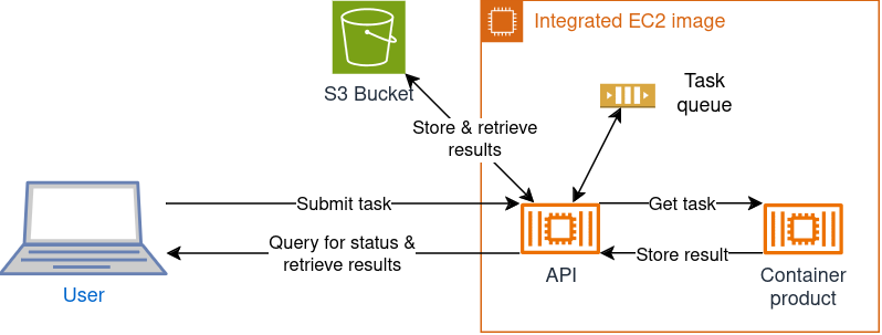
Figure 3: AWS EC2 image setup

Application programming interface (API)

The full documentation of the API endpoints will be available when you have deployed the container image on your server instance.

Figure 4: Documentation page of API with all the endpoints and direct data entry possibilities to test the endpoints and to initiate calculation tasks.

The general API structure of the current container release can be categorized in the following three endpoints:

POST request via endpoint /api/tasks

The POST request holds the following needed data:

• name of the calculation task
• basis set
• dielectric constant
• molecule geometry in xyz coordinates
• the quantum chemical approximation method, for example SCF
• the van der Waals radii of the individual atoms
• and the element definition for the individual atoms.

That’s it.

In this way you are able to send multiple calculation tasks to the high performance COSMO algorithm running on energy efficient AWS Graviton Arm processors (64 bit Linux CPU).

We also support other processor architectures. Please reach out if you would like to run COSMO calculations with other processor architectures. We can also provide containers for Intel, AMD and Nvidia CPUs/GPUs.

GET request /api/tasks

A GET request via the /api/tasks endpoint will always deliver a list of all tasks and the status of the individual task.

The list of dictionaries with each individual task has the following schema:

 1
 2
 3
 4
 5
 6
 7
 8
 9
10
11
12
13
14

[
  {
    "id": "string",
    "name": "string",
    "status": "string",
    "results": [
      {
        "type": "string",
        "url": "string"
      }
    ],
    "error_message": "string"
  }
]

One can also retrieve the list of tasks via Python with the following code snippet:

1
2
3
4
5
6

import json
import requests

r = requests.get("http://IP_ADDRESS/api/tasks")
tasks = r.json()
print(json.dumps(tasks, indent=2))

GET request /api/tasks/{task_id}

By sending a GET request to this endpoint with the specific task_id, one receives the information of either a successful response (Code 200) or an error response (Code 422).

The schema looks as follows for the successful response:

 1
 2
 3
 4
 5
 6
 7
 8
 9
10
11
12

{
  "id": "string",
  "name": "string",
  "status": "string",
  "results": [
    {
      "type": "string",
      "url": "string"
    }
  ],
  "error_message": "string"
}

And the schema for the error response is:

 1
 2
 3
 4
 5
 6
 7
 8
 9
10
11
12

{
  "detail": [
    {
      "loc": [
        "string",
        0
      ],
      "msg": "string",
      "type": "string"
    }
  ]
}

The following code snippet shows how to send a request via Python:

1
2
3
4
5
6
7

import json
import requests

task_id = "9b1b9052-61e1-43ba-98a7-44a11fe78e10"
r = requests.get(f"http://IP_ADDRESS/api/tasks/{task_id}")
tasks = r.json()
print(json.dumps(tasks, indent=2))

All tasks and results data is being stored in a S3 bucket and can be directly accessed through the AWS S3 bucket page (see Figure 5) or one can directly request the individual tasks’ data via this Python snippet (the boto3 package has to be installed):

1
2
3
4
5
6
7
8
9

import boto3

s3_client = boto3.client('s3',
                         aws_access_key_id='YOUR_ACCESS_KEY',
                         aws_secret_access_key='YOUR_SECRET_KEY')
response = s3_client.get_object(Bucket='YOUR_BUCKET_NAME',
                                Key='YOUR_OBJECT_KEY')
object_content = response['Body'].read().decode('utf-8')
print(object_content)

YOUR_OBJECT_KEY has the following path: “tasks/TASK_ID/TASK_NAME_cosmo.json”

One can also make use of the AWS CLI via the command line:

1

aws s3 cp s3://YOUR_BUCKET_NAME/TASK_ID/TASK_NAME_cosmo.json .

If no TASK_NAME was defined in the input then the results can be retrieved as follows:

1

s3://YOUR_BUCKET_NAME/TASK_ID/TASK_ID_cosmo.json

In the AWS dashboard the individual tasks folder view can be seen in Figure 5.

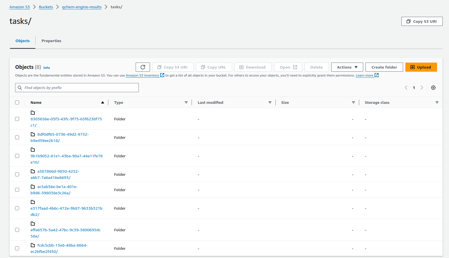Figure 5: S3 bucket view of all task folders for specific S3 bucket. The bucket name is defined by the user when setting up the container.

COSMO results data

You can get full access to all variables and parameters in the COSMO model. The results include for example:

• the number of cosmo segments and their coordinates
• the molecular surface area
• the molecular COSMO volume
• the cosmo surface charges for each segment

When retrieving the results of your calculation tasks you can get a complete and extensive overview which data is currently retrievable from the high performance COSMO implementation.

Upcoming features

The next release versions will include the sigma profiles generation endpoints so that these can directly be used for the COSMO-SAC model. Further, the first thermodynamic property endpoints will be provided for easily accessible solubility predictions.

Please reach out if you would like to set up a demo online meeting (contact at mqs dot dk).

References

[1] https://openstax.org/books/chemistry-2e/pages/10-4-phase-diagrams

[2] Jackson, J.D.; Classical Electrodynamics, Third Edition, 1999

[3] J. Tomasi, B. Mennucci, R. Cammi; Quantum Mechanical Continuum Solvation Models; https://doi.org/10.1021/cr9904009

[4] A. Klamt, C. Moya and J. Palomar; A comprehensive comparison of the IEFPCM and SS(V)PE continuum solvation methods with the COSMO approach; J. Chem. Theory Comput. 2015, 11, 9, 4220–4225; https://doi.org/10.1021/acs.jctc.5b00601

[5] W. Hackbusch; Integral Equations: Theory and Numerical Treatment, 1995

[6] E. Cancès and B. Mennucci; New applications of integral equations methods for solvation continuum models: ionic solutions and liquid crystals; J. Math. Chem. 1998, 23, 309–326.; https://doi.org/10.1023/A:1019133611148